
When building models in solid mechanics, we often have a part where there are prescribed loads but no constraints that we can reasonably apply. There are a number of different strategies that we can employ in such cases, depending on the geometry. Let’s look at how to use these different approaches and their nuances.
A Solid Mechanics Problem
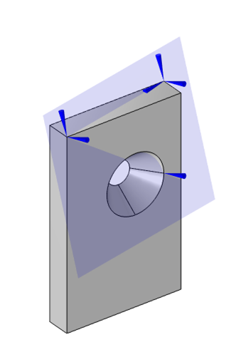
We will start by considering a simple model of a flat plate with a hole through it — a classic problem in solid mechanics. Let’s assume that there are equal and opposite forces applied at the top and bottom. Imagine, perhaps, that this part is connected to some cables via some fixturing and put in tension.
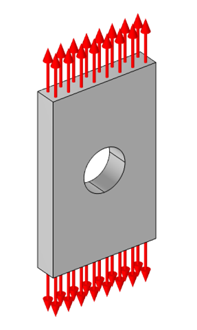
Free-body diagram of a flat plate with a hole in the center, under a tension load.
Although we could build a model of the fixturing and the cables, and a model of whatever the cables are connected to, this is likely much more effort than we want to expend. We really just want to focus our analysis on this one part of a larger system, so it makes sense to approximate all of these other parts as a boundary load that is normal to the ends of the plate.
Now, we intuitively know that a part with equal and opposite forces on it will not experience any accelerations, so although the part will deform, it won’t be in motion. That is, we can say with confidence that a stationary solution to this problem exists, even if we don’t know where the part is or how it is oriented. That is, the applied forces could be aligned with any arbitrary direction and the solution in terms of the stresses and strains would still be the same.
Now, when we solve a solid mechanics problem via the finite element method, we aren’t directly solving for the stresses or strains. Instead, we solve for the displacements (or deformations) from the undeformed state. The stresses and strains are computed from the displacement field. For the purposes of this blog post, it is sufficient to address solely the linear case, but if you’re interested in some more advanced topics, see the following blog posts:
To get a solution for the deformations, we do need to introduce a set of constraints on the displacement field, and these must be sufficient to constrain all free-body displacements and rotations, but they cannot affect the stresses and strains. This blog post will describe various ways in which this can be achieved, depending on the geometry that we’re dealing with.
Using Symmetry Planes
For this geometry, the experienced structural analyst will immediately see that there are three planes of symmetry that can be exploited. We can draw the part aligned with the global Cartesian coordinate system and use partitioning along workplanes parallel to the xy-, yz-, and xz-planes. This reduces our model to a 1/8 submodel of our original model. We apply the symmetry condition to the three faces along these planes, and this will have the effect of completely constraining our part. In addition, this has the beneficial side effect of reducing the computational size of our model.
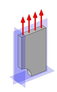
Exploiting symmetry along three orthogonal planes fully constrains the model.
Let’s think about exactly how these three symmetry conditions constrain the part. The symmetry condition imposes that there be no displacement in the normal direction to the selected (planar) boundaries. Thus, the symmetry condition applied on the face parallel to the xy-plane will impose the condition that this face has zero displacement in the z direction, and that there can be no rotations about the x-axis and the y-axis.
Next, the symmetry condition on the yz-parallel face imposes the additional conditions that there can be no displacement in the x direction and no rotation about the z-axis. The rotation around the y-axis is once more constrained, but this is not a problem.
Finally, the symmetry condition on the xz-parallel face imposes the additional constraint of no displacement in the y direction.
Thus, we have applied a set of three orthogonal constraints on the displacements and rotations, so the part is sufficiently constrained and the model can be solved. To visualize the results, it is helpful to use a set of three Mirror 3D datasets, which can mirror any dataset about a plane such that the complete part can be visualized.
Parts with No Symmetry
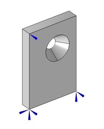
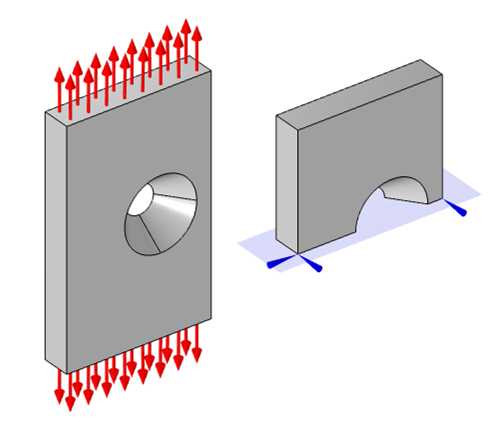
Unfortunately, we usually aren’t so lucky as to have a part with three planes of symmetry. Let’s modify our part by introducing a taper to the hole, and changing its location, as shown below.
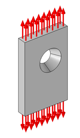
Free-body diagram of a flat plate under tension with an off-centered tapered hole.
There is no way to exploit any symmetry in this case, so what can we do? There are actually four different approaches we could take!
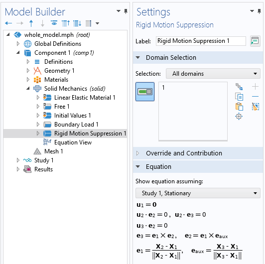
Applying the Rigid Motion Suppression feature to all domains to constrain displacements and rotations.
The first, simplest approach is to use the Rigid Motion Suppression domain constraint feature. This feature simply needs to be applied to any one, or all, subdomains of the model, and it will apply a set of constraints behind the scenes that removes all rigid-body displacement and rotation. All we need to do is apply this feature and the model will solve.
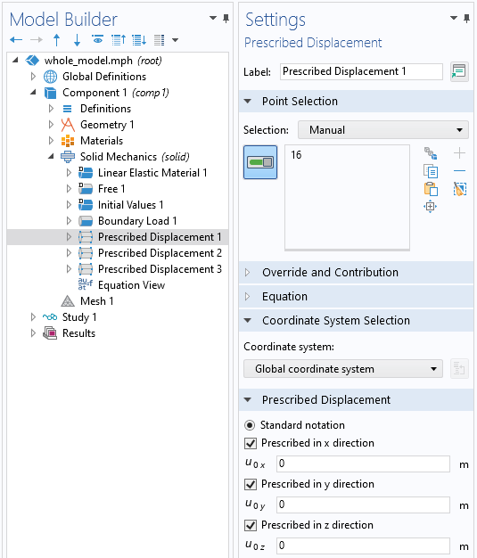
A Prescribed Displacement point condition that constrains all free-body displacements.
The second approach is to manually constrain displacements and rotations via a set of three different point constraints. To do so, begin by choosing a point on the geometry, and impose a Prescribed Displacement condition on that point that sets the x-, y-, and z-displacements to be zero.
Although the point that we choose could be arbitrary, we will see shortly that it is best to choose a point at one of the corners of this rectangular-shaped part. This single constraint is sufficient to remove all rigid-body displacement and will have no effect on the stress and strain fields.
Visualization of three point displacement constraints that constrain all free-body rotations and displacements, but have no effect upon the strain field.
Next, we need to remove rotations about three orthogonal axes. This can be a bit trickier, although in this case, we are lucky in that our geometry is aligned with the global Cartesian axes. So, we can start from our fully constrained point and look along the Cartesian directions.
Let’s first look along the x-axis from this point until we find another point. There, we apply another Prescribed Displacement condition to remove a rigid-body rotation, but we need to make sure that we do not impose a constraint that will affect the strains and stresses. Another way of saying this is that we don’t want to impose a constraint on the distance between these two points. So, at this second point, we will constrain the displacement in the y– and z directions, but leave the x-displacement unconstrained. This constraint removes rotation about the z-axis and the y-axis, respectively. The part is now only free to rotate about the x-axis, and we can remove this freedom with one more point constraint.
If we go back to our original fully constrained point, we can now look along either the y-axis or the z-axis until we find a point. Let’s search along the z direction, and, once we’ve found a point, we can apply a Prescribed Displacement condition such that there is zero displacement in the y direction. This will prevent rotation of the part about the x-axis. Again, we need to make sure we aren’t constraining the distance between any of these points. If you do so by accident, you’ll see locally high stresses.
This second approach is actually a manual implementation of what is being done automatically by the first approach. It might, though, raise a question: What happens when we don’t have three points aligned with the Cartesian axes? If using the first approach, of the Rigid Motion Suppression, that feature will automatically be able to select any three points that form a plane and apply a consistent set of constraints. Let’s also look at how we can use any three points, as long as they describe a plane.
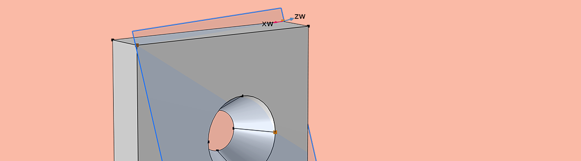
In our third approach, let’s work with the same geometry, but constrain using three points that aren’t aligned with the Cartesian axes. We will need to first define a Workplane, then define a Coordinate System using that workplane, and finally use that Coordinate System within our Prescribed Displacement conditions.
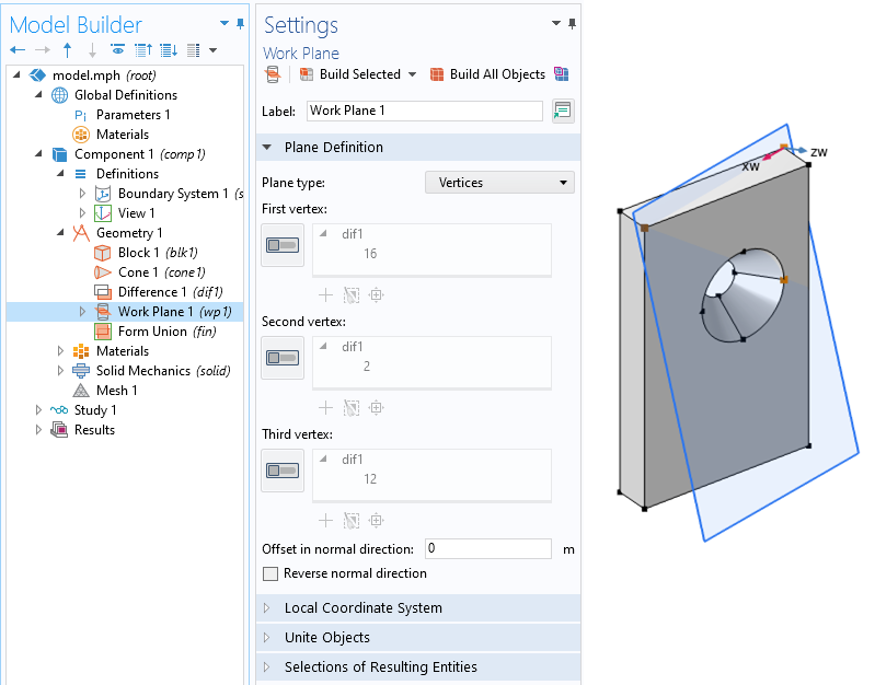
Three arbitrary points can be used to define a new workplane.
Start by defining a new Workplane within the Geometry, of Plane type Vertices, and choose three points that define a plane and that aren’t colinear. Note that the first two vertices that we select will define the first local axis of this plane. Next, define a Coordinate System from Geometry. Set the Frame of this coordinate system to be Spatial and choose the new Workplane in the System from Geometry setting.
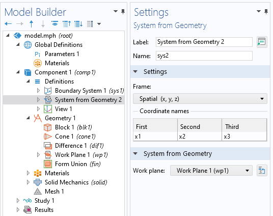
Defining a coordinate system based upon a workplane.
Then, as before, add three Prescribed Displacement point conditions, and for each, set the coordinate system to the System from Geometry. These three points should correspond to the three points selected within the Workplane feature. At the first point, constrain all three displacements. At the second point (the one that defines the first local axis), constrain the displacement in the second and third directions. At the third point, constrain displacement in the third axis (normal to the plane) direction. The advantage of this approach is that it doesn’t require the part to be aligned with the Cartesian axes. Again, the Rigid Motion Suppression feature provides the equivalent capability.
Visualization of three point displacement constraints that constrain all free-body rotations and displacements, in a coordinate system defined by these three points.
The fourth approach addresses the special case of a geometry that does not have three points that define a plane. This can occur when we are dealing with imported mesh files, as in this model of a vertebrae, which does not have any points defined on the original mesh. Although it is possible to manually create vertices on an imported mesh, and it is possible to partition edges of a geometry to introduce additional points, it is worth knowing about this last alternative.

Using the Spring Foundation feature also constrains displacements and rotations, but does not affect the solution if the spring constant is small enough.
In this fourth approach, we use the Spring Foundation domain feature and apply it to all domains of the model. This feature introduces an artificial additional stiffness at every degree of freedom of the structural model, relative to its undeformed position. The magnitude of this spring constant is a tuning factor within the model. If it is too small, then it will not provide sufficient numerical stiffness, and the model will not solve, but it shouldn’t be too large either, as this also affects the results. In practice, start with a very low value, and make it bigger until the model solves. Although there are only very rare conditions where this technique is strictly necessary, it is still worth knowing about.
Parts with Partial Symmetry
Let’s also consider the quite common situation of a part with some symmetry, in which case the Rigid Motion Suppression feature cannot be used.
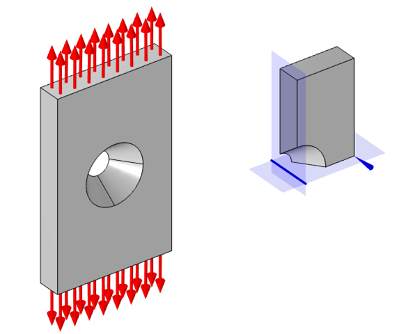
Exploiting half-symmetry requires two point displacement constraints that remove translation in the plane and rotation about the axis normal to the plane.
For the case of a single symmetry plane in the model (or two parallel planes of symmetry), we have to choose two points on the plane and use the Prescribed Displacement point condition to constrain them such that there is no displacement in that plane and no rotation about the normal to that plane. If there are two planes of symmetry at an angle to each other, then choose a single point on one of the planes, and constrain it such that it cannot move in the direction described by the intersection line of the two planes.
With two planes of symmetry, remove translation along the intersection line of the planes via a single point constraint.
In terms of presenting the results of such models, it is also good to know how to center the visualization of the displacements. Suppose we want our model to be visualized with the displacement centered about the hole. What we can do is introduce an average component coupling operator and define it over the boundaries of the hole. Then, when visualizing the displaced results, we can subtract out this averaged location in the Deformation subfeature, as shown in the screenshot below.
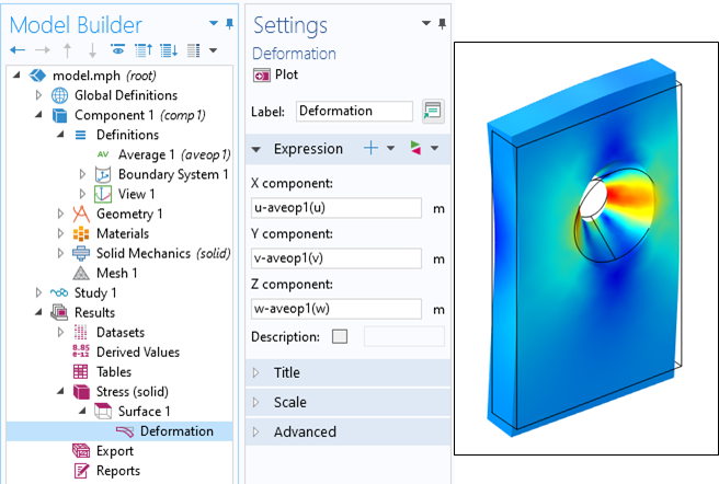
Using the average operator to recenter the visualization of the displacement about the center of the hole.
Concluding Thoughts on Modeling Parts Without Constraints
In summary, we have shown a set of techniques to use for modeling 3D parts where we only have a set of balanced loads, but no constraints. The simplest approach is to use the Rigid Motion Suppression feature, but we sometimes need to constrain via a set of points due to other symmetry conditions.
For the case of 2D structural models, a similar but simpler approach is applied. For parts without symmetry, one point has to be fully constrained in the xy-plane and another point must be constrained to prevent rotation about the out-of-plane z-axis. For a 2D model with one plane of symmetry, or parallel symmetry planes, only one point displacement constraint is needed to prevent motion along the symmetry plane. For a 2D model with intersecting symmetry planes, no additional constraints are needed. For the case of 2D axisymmetric models, only the displacement along the z direction (parallel to the axis of symmetry) must be constrained at any single point.
These techniques are particularly useful when dealing with problems involving thermal expansion, and can be used in any study type, including stationary, time-domain, frequency-domain, or eigenfrequency. These methods are a powerful tool for all structural analysts.


Comments (4)
Robert Gustavsson
January 12, 2021Thank you for this post! Very useful on how to approach this issue. I can use this information already today 🙂
However, the spring constant tool could use some more instructions on how to find the proper stiffness instead of shooting in the dark, i.e. maybe there is a rule-of-thumb to use?
Walter Frei
January 12, 2021 COMSOL EmployeeHello Robert,
Yes, a quick hand-calculation based upon the overall size of the system and expected deflections is also a good estimator.
Temesgen Kindo
January 26, 2021Thanks Walter for the nice summary.
@Robert, I just wanted to add to Walter’s response to your question. He provided a way to estimate the spring stiffness prior to running the simulation. I would like to comment on how to check, after the simulation, if you had picked an appropriate stiffness. When you postprocess the reaction force coming from the added spring, it should be orders of magnitude smaller than the applied forces (not net force as that is often zero, but each) or reactions forces from real supports. If the smallest applied force or real reaction is F, you may live with an artificial spring reaction of F/1000 but a reaction of F/10 may be too much.
Robert Gustavsson
June 17, 2022@Temesgen, what parameter should I plot to check the spring reaction?