

When buying a new car, the sounds and feelings you experience when closing its door give a subtle yet important contribution to your first impression. The doors are sensitive to vibrations and, depending on their design and structure, this causes different sounds when you close the doors of different cars. The ability to reduce these vibrations in car doors is important for the driving experience. At high speeds, the fluid flow may cause vibrations in the door and side window, which may propagate into the passenger compartment, and even the trim panel and other interior parts, causing annoying noise. Some people can get extremely frustrated (no names mentioned) just from the noise of a loose belt buckle vibrating against the B-pillar while driving. I cannot imagine what would happen if a trim panel would start giving off noise!
An important part of the design, regarding vibrations at high speeds, is the aerodynamics of a car. Modeling and simulation can be used to estimate the flow and pressure field around a car with reasonable accuracy. The fluctuating pressure exerted by the flow can be used as surface loads in a structural analysis. In this context, it is important that the forces exerted by the air at high speeds are estimated regarding not only magnitude but also frequency.
In this blog post, we look at the use of large eddy simulation (LES) models to predict the transient forces that the airflow generates on the door and side mirror of a sports car at high speed. The forces are then used as loads in a structural analysis.
Why a sports car? Because it is more fun, of course! And since I will probably never own a supercar, modeling one may give me enough satisfaction for a while…
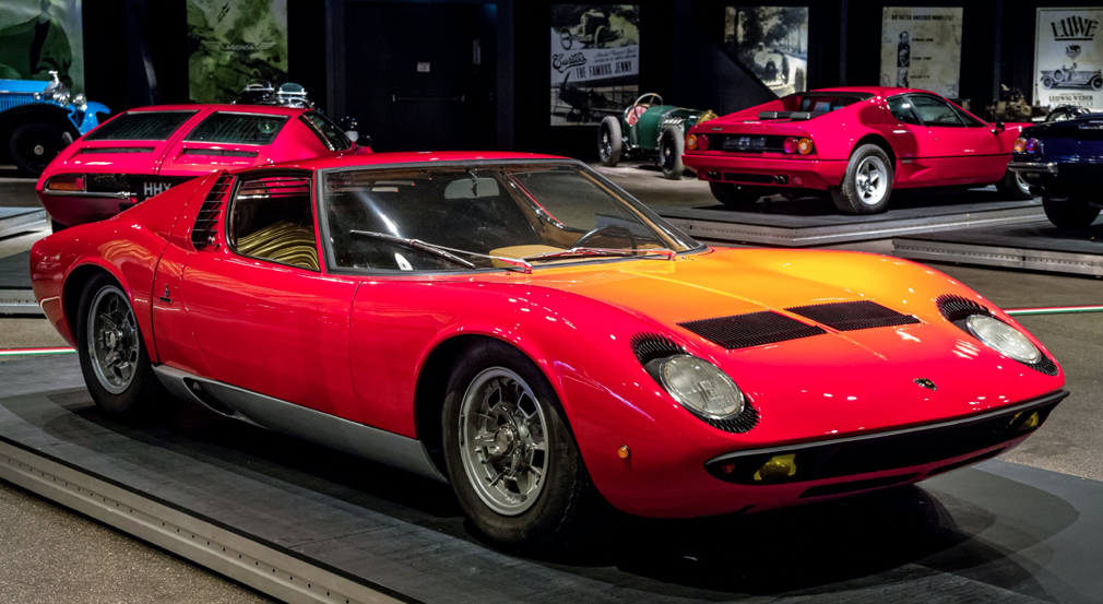
The Lamborghini Miura® is considered to be the first supercar. It was produced from 1966 to 1973. Here is the 1967 P400 model. To the right in the background we can see the rear of another classic supercar, the Ferrari® 512 BB, released in 1972. To the left in the background is the rear of a De Tomaso Mangusta®, with its classical wing-style rear windows, also released in 1967. Image by joergens.mi — Own work. Licensed under CC BY-SA 3.0, via Wikimedia Commons.
Editor’s note: Lamborghini and Miura are registered trademarks of Automibili Lamborghini S.p.A. De Tomaso Mangusta is a registered trademark of De Tomaso Automobili Limited. Ferrari is a registered trademark of Ferrari S.P.A. No sponsorship, endorsement, affiliation, or other connection is implied with respect to the owners of such marks.
The Large Eddy Simulation Model
The advantage of the LES model is that it can give accurate estimates of the flow’s fluctuation with time. This also means that it can estimate the forces on the surface of the body of the car as a function of time. We want to use these time-fluctuating forces as loads in the structural analysis of the door and mirror, but then by transforming these loads to the frequency domain using fast Fourier transform (FFT). This should result in an estimate for the risk of vibrations in the doors and mirrors by looking at the eigenmodes that are excited by the loads.
The flow field around the doors and mirrors depends on the shape of the car. To get an accurate flow field, we need to model the whole car. In addition, it is more fun to model the whole car, at least if we can afford the computational cost.
The fluid flow analysis is somewhat complex, because we need to get decent initial conditions for the LES model. This involves solving a Laplace equation for potential flow, using the solution from the potential flow as the initial condition for a RANS (Reynolds-averaged Navier–Stokes) simulation, and then in turn using the results from the RANS simulation as the initial condition for the LES model. The first step is performed in order to reduce the number of iterations for the RANS simulation. In this case, we do not want to define a separate RANS interface and an LES interface, since this would duplicate the number of degrees of freedom. Instead, we change the properties of the RANS interface to LES. This is not the most elegant way of setting up the model in the COMSOL Multiphysics® software, but it is the least computationally expensive way. The figure below shows the model tree for the fluid flow model.
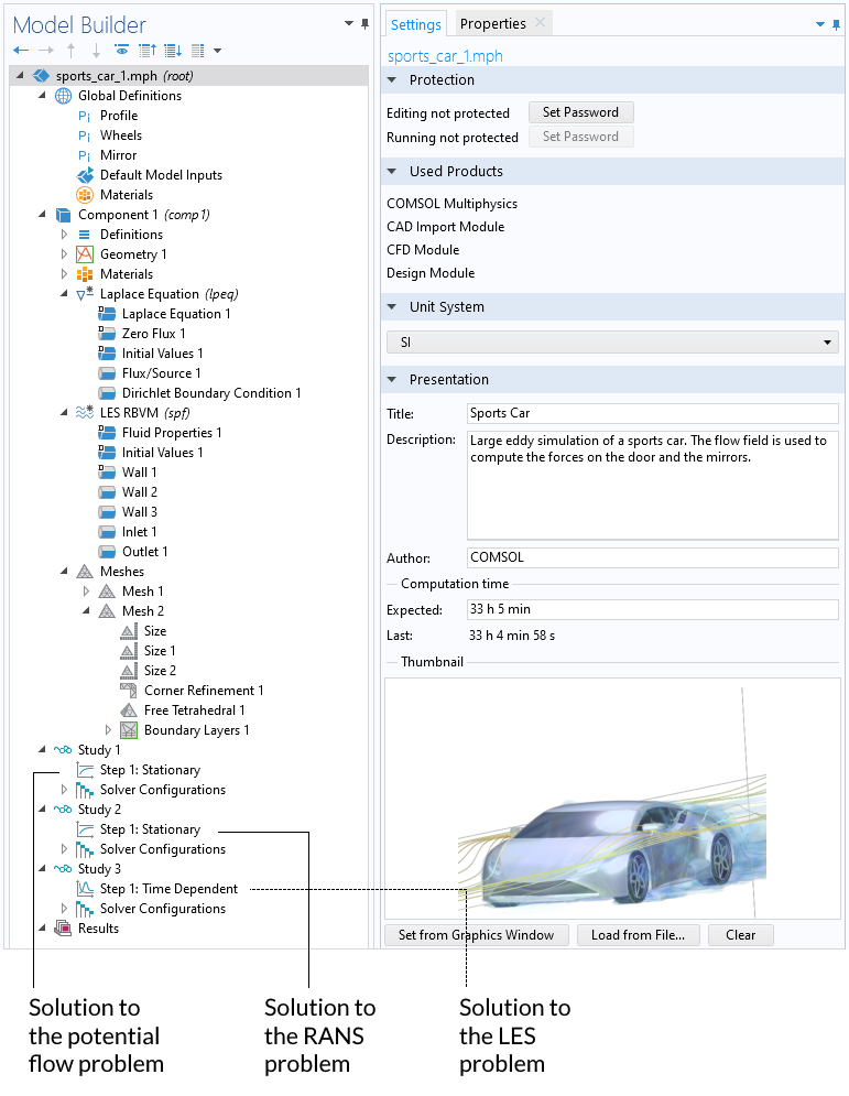
The model tree for the fluid flow problem.
The bounding box for the air domain around the car has to be large enough so that we hopefully know something about the flow or about the pressure at the boundaries in order to define the boundary conditions. This in turn determines what the mesh should look like. We need a boundary layer around the car. We also have to allow some element growth away from the car to reduce the size of the problem. The mesh is shown below.

The mesh in the air domain and a magnification of this mesh closer to the car. At the surface of the car, a boundary layer mesh is automatically created.
The figure below shows the flow behind the car. We can see that the flow trail reaches very far behind the car. This trail must become quieter and smoother in order to set a boundary condition behind the car, hence the very long air domain behind the car.

The disturbance in the flow field behind the car running at 180 km/h reaches very far behind the car, hence the need for a long air domain.
The areas around the mirror and the upper part of the door, the side window, are subjected to the highest relative flow. The figure below shows the flow from the front and rear, with the areas around the side door magnified. The drag coefficient of this homemade car is computed to 0.19 by the model, which is a low but realistic value.
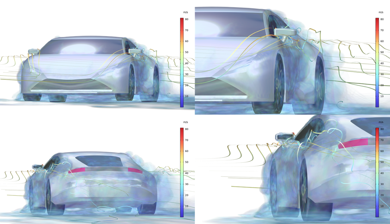
The flow field around the car and a magnification close to the side doors.
The Structural Model Using a One-Way FSI Study
We can run a first initial test example in the time domain using the forces exerted by the flow. In addition to giving us a grasp of the deformations that we can expect on the mirror, it should also result in some cool animations. (The impact of nice animations should never be underestimated!) Below, we can see how the flow deforms the mirror. The deformations are exaggerated by a factor of 50 for visualization purposes.
Vibration of the mirror caused by the flow. Note that the deformation is exaggerated by a factor of 50, otherwise we would not see how the mirror moves.
In the time-domain analysis, it is however assumed that the initial conditions are zero. Also, due to the random nature of the loading, a good time-domain analysis would have to be performed over a very long simulation time in order to give reliable results. We need to use a more sophisticated approach.
The next step is to define a structural model in the frequency domain in order to see how different details in the door may vibrate. We can do this by first using FFT to transfer the fluctuating forces caused by the flow from the time domain to the frequency domain. In this case, we use a time range for the flow simulation of 0.7 s. The last interval of 0.1 s, from 0.6 to 0.7, shows that the flow is already stable. This is after 35 m of speeding at 180 km/h, corresponding to 8 car lengths. Since we are now sampling a period of 0.1 s, the resolution in the frequency domain will be 10 Hz. A longer sampling interval could be used to increase the frequency resolution. The total force in the side window shows spikes at 90 Hz and 160 Hz. The side mirror has a major spike at 50 Hz, and a plateau in the range 70-90 Hz. If the peaks in the frequency spectra would coincide with important natural frequencies of the structure, there is a risk of amplification due to resonance.
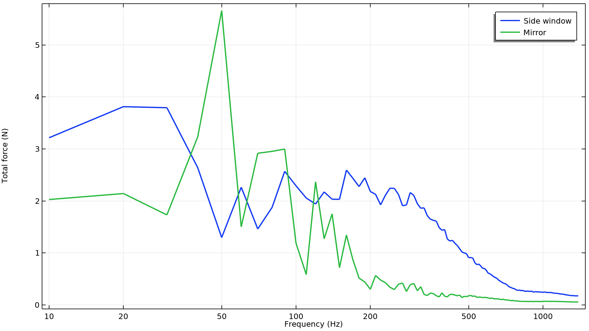
In this graph, we can see the total forces on the side window and the mirror as a function of frequency. Note that the static load from the mean flow is not included.
The image below shows the model tree for transferring the fluctuating forces to the frequency domain and for performing the structural analysis to find the response.
Model tree for the structural analysis in the frequency domain. Study 4 transfers the wind loads from the time domain to the frequency domain. Study 5 runs the frequency-domain study with the excitation from the wind load. The solution is then transferred back to the time domain in the last study step.
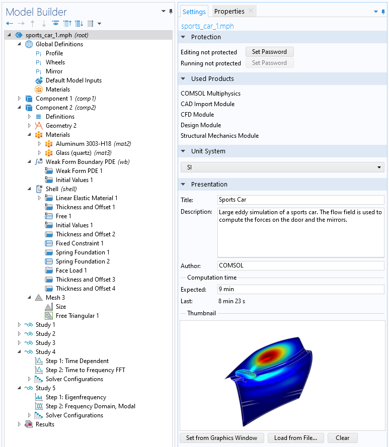
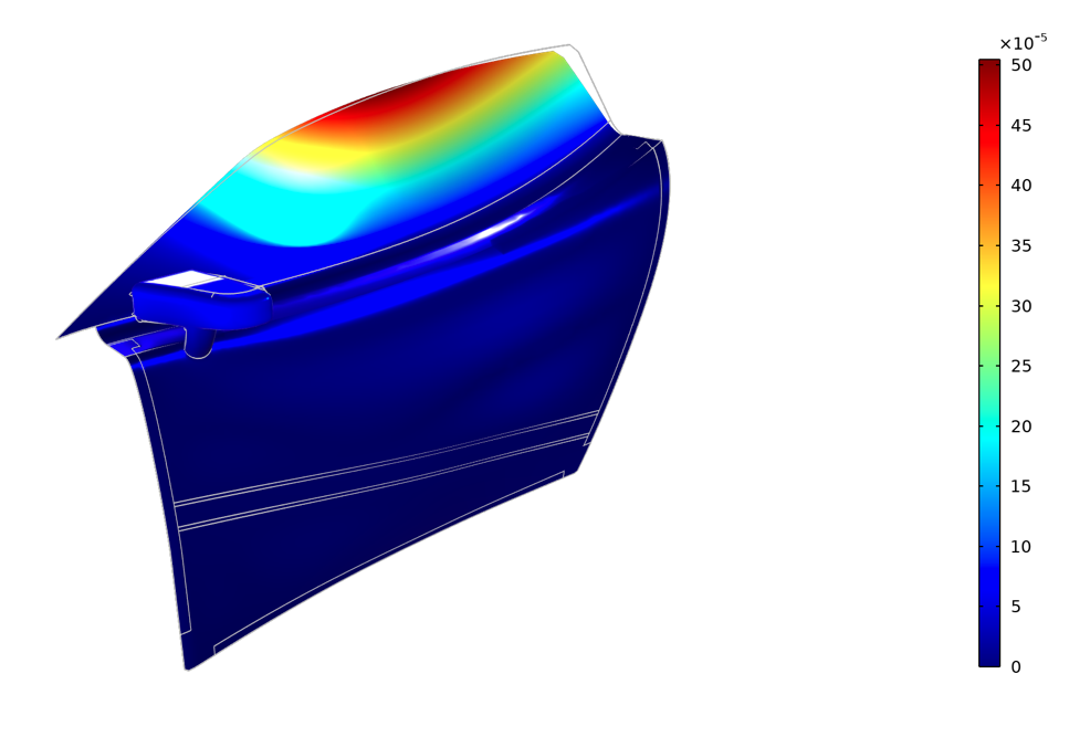
Once we have transformed the stresses in the fluid to the frequency domain, we can apply them as loads on the door and the mirror. In this analysis, we can use the full geometry of the side door, but we do not have to account for the rest of the car. An interesting excited mode is shown below at 90 Hz. We can see that the side window vibrates with nodes at the window edges, and the upper part of the door vibrates with nodes at the side-impact door beam and the frame of the door. Such a mode could be difficult to damp completely. This means that we would probably hear the wind at this frequency.
The response to the fluid load at 90 Hz. The whole side window and the side door vibrate almost uniformly over a large portion of their surfaces.
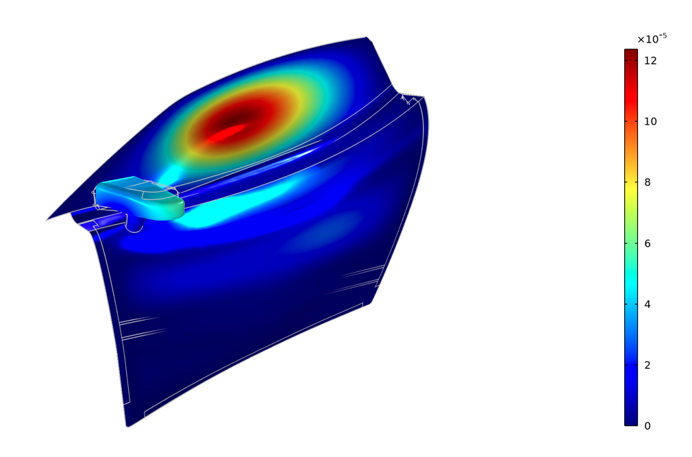
Another interesting mode is found at 50 Hz. Here, both the inside structure of the door and the side mirror vibrate in response to the fluid loads on the exterior surfaces. However, we can hope that the trim panel attached to the metal may help with damping the vibrations on the inside structure.
The response at 50 Hz shows that both the inner metallic structure of the side door and the side mirror vibrate. This is probably damped by the trim panel attached to this surface.
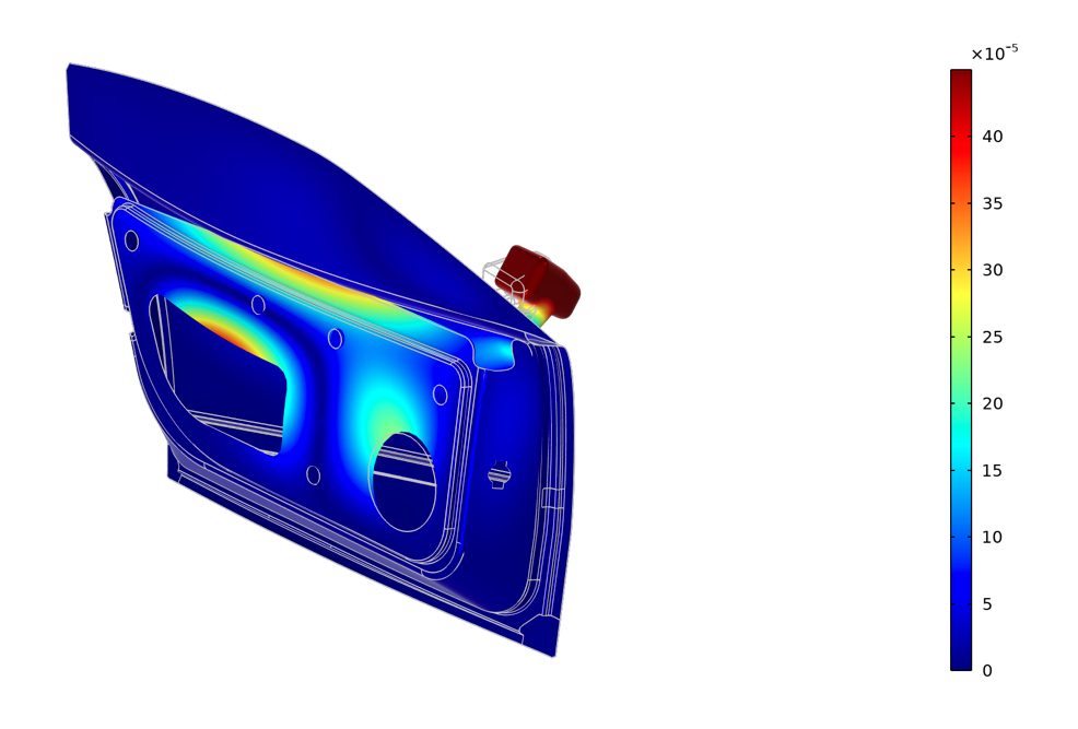
The worst case of fluttering noise occurs when you have to roll down the window slightly. You may need to do that when somebody performs flatology studies in the car or if somebody lights a cigar. Then the upper edge of the window is not constrained and the eigenmodes show that the whole side window flaps. Vibrations of the upper edge of the side window occur at 20 Hz.
The response at 20 Hz generates vibrations of the upper-rear corner of the side window.
Extension of the Wind Load on a Sports Car Model
The car body has several simplifications. For example, the different parts of the body are assumed to be assembled perfectly, with no gaps nor misalignments between different body panels. In reality, the body of a real supercar is full of small gaps between body panels and doors, of the order of magnitude of a mm. These gaps may induce some additional turbulence. Another simplification here is that the wheels do not rotate in the CFD model. This should also cause turbulence. The structural analysis assumes that the door is constrained to the frame of the car with no displacements. In reality, the frame of the car also vibrates, mainly due to the road’s roughness propagating through the drive train and the suspension of the car to the frame and then to the doors.
Despite the simplifications, the model is still quite sophisticated and can very well be used as a starting point for a more accurate model. An extension of the model could include the windshield and the rear window and perform a complete analysis of the vibration of the window, which is the main source of noise. In addition, we could use the vibrations calculated using the FSI study as boundary conditions in an acoustics study of the car compartment. This would include a detailed geometry of the car compartment, such as the door trims, seats, carpets, instrumentation, etc. However, that is a topic for another blog post!
Next Step
Want to try performing an LES study of a car mirror and door? Click the button below to access the model file.

Comments (1)
Jay Puckett
December 21, 2022Very nice example, thanks. Just a suggestion is to provide the .mph with and without results for download to enable reviewing without the large file size.