
We live in a three-dimensional world — or maybe four-dimensional, if you consider space–time. Still, in engineering analysis, it is common to use 2D approximations to save both modeling and computational resources. In this blog post, we take a look at when and how it is possible to study problems in the field of solid mechanics using 2D formulations.
Table of Contents
- What Is 2D?
- Different 2D Formulations for Solid Mechanics
- Constitutive Models
- Which Formulation Should I Choose?
- Why Do Transverse Stresses Occur?
- What About In-Plane Stresses?
- Inelastic Strains
- A Note on Equivalent Stresses
- A Note on Fracture Mechanics
- 1D Theories
Editor’s note: This blog post was updated on December 16, 2022, to reflect new features and functionality in version 6.1 of the COMSOL Multiphysics® software.
What Is 2D?
There is not much in real life that is actually two-dimensional. When we, for example, study the electromagnetic fields around a cable cross section in 2D, we are actually saying: “This cable is straight and long. Sufficiently far from the ends, the fields depend only on the location in this cross-sectional plane.” For most physical problems, this is the idea: In a 2D approximation, we study a cross section of a long, straight object, ignoring end effects.
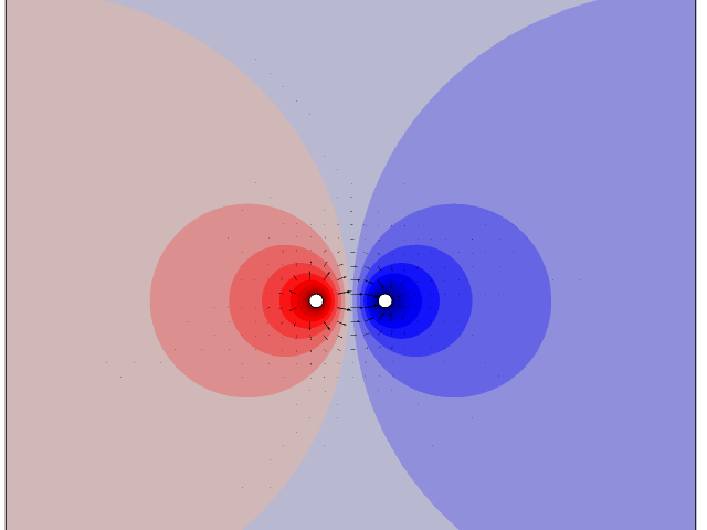
The electric potential (color code) and electric field (arrows) around two long cables with different potentials, as computed in 2D.
The cross section is representative of a situation in which the cables are long, straight, and parallel.
Why Is Solid Mechanics Special?
In the field of solid mechanics, there are more possibilities for 2D states than a very long extrusion. We can, for example, consider a thin, flat plate, loaded only in its plane, as two-dimensional. What is then so special with solid mechanics that makes this possible?
Consider analyzing the same plate for heat transfer. In that case, convection and radiation from the large surfaces will occur in the out-of-plane direction. Then, the temperature gradient in the thickness direction is important. Thus, a 2D approximation for heat transfer in thin plates is more difficult. Similar reasoning can be applied to many other physical phenomena.
In the case of solid mechanics, there is also an effect in the out-of-plane direction. The thin plate will, in general, deform in the transverse direction. For example, it will get thinner if you stretch it. However, that does not directly affect the solution to the 2D problem. The thickness change is a result that can be computed a posteriori, in case you are interested. This will be discussed in more detail below.
Different 2D Formulations for Solid Mechanics
In the following section, it is assumed that 2D means the xy-plane, and that z is the out-of-plane direction. The displacements in the xy-plane are called u and v respectively, and w is the displacement in the z direction.
It should be noted that if there is no coupling between in-plane and out-of-plane action (for example, when Poisson’s ratio is zero for a linear elastic material), then all formulations will be identical.
Plane Strain
Plane strain is the only one of the 2D solid mechanics formulations that does not contain approximations. A state of plane strain will exist in an object that is constrained in the z direction between two rigid walls. This is also the formulation that conceptually has the best correspondence to 2D formulations in other physics fields. The object does, however, not have to be “long” in the z direction. This is a fundamental difference from the 2D approximations for most other physics fields.
The assumptions are simple: No displacement in the z direction.
{\begin{array}{*{10}{l}}
u&=&u \left ( x,y \right ) \\
v&=&v \left ( x,y \right ) \\
w&=&0
\end{array}}
{\ }
\]
This can equivalently be expressed in terms of strains:
{\begin{array}{*{10}{l}}
u&=&u \left ( x,y \right ) \\
v&=&v \left ( x,y \right ) \\
\varepsilon_{zz}&=&\varepsilon_{xz}&=&\varepsilon_{yz} &=& 0
\end{array}}
{\ }\]
Note that in order to completely avoid end effects, it is actually assumed that the boundary conditions at the rigid walls are of a roller type, so that the displacement in the xy-plane is not inhibited. If this is not the case, then we are back in the situation where we study a long object, far from the ends.
Plane Stress
In a plane stress formulation, the assumption is that the three stress tensor components relating to the z direction are zero. This is a good approximation for thin plates, but it is fully true only in the limit when the thickness approaches zero.
{\begin{array}{*{10}{l}}
u&=&u \left ( x,y \right ) \\
v&=&v \left ( x,y \right ) \\
\sigma_{z}&=& \sigma_{xz}&=&\sigma_{yz}&=& 0
\end{array}}
{\ }\]
On a free surface, a local state of plane stress always prevails, since this is exactly the boundary condition. This is why the plane stress assumption works so well — It is exactly true on the two opposite sides of the plate, and as long as the thickness is small, no significant z direction stresses will develop in the interior.
Generalized Plane Strain
Unfortunately, there is no unique definition of generalized plane strain, but it usually means that some of the assumptions for the ordinary plane strain formulation are relaxed. Assume that the entire strain tensor is allowed to be nonzero, but still only depends on x and y. Then the following displacement field can be shown to give such a strain tensor:
{\begin{array}{*{10}{l}}
u&=&u \left ( x,y \right ) – \frac{a}{2} z^2 \\
v&=&v \left ( x,y \right ) – \frac{b}{2} z^2 \\
w&=&\left (ax + by +c \right )z
\end{array}}
{\ }
\]
Here, a, b, and c are constants. The infinitesimal out-of-plane strains will then be
{\begin{array}{*{10}{l}}
\varepsilon_{zz}&=&ax +by +c \\
\varepsilon_{xz}&=&\varepsilon_{yz}&=&0
\end{array}}
{\ }
\]
In the z = 0 plane, where the analysis is performed, w is zero. Thus, there are still only two components of the displacement field, u and v, to be solved for. There are, however, three new unknowns, a, b, and c. In a common interpretation of generalized plane strain, only the coefficient c is used. Physically, this means that the long object is allowed to expand axially in the z direction. If the parameters a and b are also included, the extrusion is also allowed to bend with a constant curvature. The values of a, b, and c are determined by the assumption that no net axial force or bending moments act on the cross section; that is, the ends are free.
When you select the generalized plane strain option in COMSOL Multiphysics, you have the possibility to select between the pure axial extension assumption and the inclusion of bending.
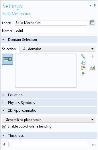
Selecting generalized plane strain.
There are also other formulations that are sometimes called generalized plane strain. For example, the out-of-plane shear strains, \varepsilon_{xz} and \varepsilon_{yz}, can be allowed to be nonzero. Such a formulation, together with \varepsilon_{zz} = 0, is used in the 2D version of the Elastic Waves, Time Explicit interface.
Constitutive Models
Under the assumption of linear elasticity, Hooke’s law can be specialized for plane strain and plane stress. The full 3D form of Hooke’s law is
{\begin{array}{*{10}{l}}
\sigma_x &=& \frac{E}{1+\nu} \left( \varepsilon_{xx} +\frac{\nu}{1-2 \nu} \left ( \varepsilon_{xx} + \varepsilon_{yy} + \varepsilon_{zz} \right )\right ) \\
\sigma_y &=&\frac{E}{1+\nu} \left( \varepsilon_{yy} +\frac{\nu}{1-2 \nu} \left ( \varepsilon_{xx} + \varepsilon_{yy} + \varepsilon_{zz} \right )\right ) \\
\sigma_z &=&\frac{E}{1+\nu} \left ( \varepsilon_{zz} +\frac{\nu}{1-2 \nu} \left ( \varepsilon_{xx} + \varepsilon_{yy} + \varepsilon_{zz} \right )\right ) \\
\tau_{xy} &=& 2G \varepsilon_{xy} \\
\tau_{yz} &=& 2G \varepsilon_{yz} \\
\tau_{xz} &=& 2G \varepsilon_{xz} \\
\end{array}}
{\ }
\]
Here, E is Young’s modulus, ν is Poisson’s ratio, and G is the shear modulus.
Plane Strain
The plane strain case is trivial; it is just necessary to remove the three strain components that are zero from the 3D formulation,
{\begin{array}{*{10}{l}}
\sigma_x &=& \frac{E}{1+\nu} \left( \varepsilon_{xx} +\frac{\nu}{1-2 \nu} \left ( \varepsilon_{xx} + \varepsilon_{yy} \right )\right ) \\
\sigma_y &=&\frac{E}{1+\nu} \left( \varepsilon_{yy} +\frac{\nu}{1-2 \nu} \left ( \varepsilon_{xx} + \varepsilon_{yy} \right )\right) \\
\sigma_z &=&\frac{E \nu}{(1+\nu)(1-2 \nu)} \left( \varepsilon_{xx} + \varepsilon_{yy}\right ) &=& \nu \left ( \sigma_x + \sigma_y \right )\\
\tau_{xy} &=& 2G \varepsilon_{xy} \\
\tau_{yz} &=& 0 \\
\tau_{xz} &=& 0 \\
\end{array}}
{\ }
\]
Plane Stress
For the plane stress case, the fact that \sigma_z = 0 can be used to eliminate \varepsilon_{zz}, giving
{\begin{array}{*{10}{l}}
\sigma_x &=& \frac{E}{1-\nu^2} \left( \varepsilon_{xx} +\nu \varepsilon_{yy} \right) \\
\sigma_y &=& \frac{E}{1-\nu^2} \left( \varepsilon_{yy}+\nu \varepsilon_{xx} \right) \\
\sigma_z &=& 0 \\
\tau_{xy} &=& 2G \varepsilon_{xy} \\
\tau_{yz} &=& 0 \\
\tau_{xz} &=& 0 \\
\end{array}}
{\ }
\]
The transverse strain (thus the thickness change) can then be computed from the solution as \varepsilon_{zz} = – \frac {\nu} {1-\nu} (\varepsilon_{xx} + \varepsilon_{yy}).
In the COMSOL Multiphysics® software, this formulation is not used, however. Instead, the full 3D Hooke’s law is used together with an extra unknown field for \varepsilon_{zz}. This, of course, adds to the total problem size, but the advantages are huge: There is no need to consider special plane stress forms for all material models, and we do not have to modify, for example, thermal expansion and similar features. If you plot the transverse stress, \sigma_{z}, you will however notice that the value is not identically zero, since it is computed from the strain fields using Hooke’s law.
Generalized Plane Strain
This case is somewhat more complicated. When the assumptions for the out-of-plane strains are injected in the constitutive relation, the stress components become explicitly dependent on the coordinates x and y through the coefficients a, b, and c.
{\begin{array}{*{10}{l}}
\sigma_x &=& \frac{E}{1+\nu} \left( \varepsilon_{xx} +\frac{\nu}{1-2 \nu} \left ( \varepsilon_{xx} + \varepsilon_{yy} + ax +by +c \right )\right) \\
\sigma_y &=&\frac{E}{1+\nu} \left( \varepsilon_{yy} +\frac{\nu}{1-2 \nu} \left ( \varepsilon_{xx} + \varepsilon_{yy} + ax +by +c \right )\right) \\
\sigma_z &=&\frac{E}{1+\nu} \left( ax +by +c +\frac{\nu}{1-2 \nu} \left ( \varepsilon_{xx} + \varepsilon_{yy} + ax +by +c \right )\right) \\
\tau_{xy} &=& 2G \varepsilon_{xy} \\
\tau_{yz} &=& 0 \\
\tau_{xz} &=& 0 \\
\end{array}}
{\ }
\]
Incompressible Materials
The lesser the degree of compressibility, the stronger the coupling between in-plane and out-of-plane action. In particular, many models for plasticity, creep, and hyperelasticity assume incompressibility. When working with such material models, the effect of the selected 2D assumption is particularly strong.
Which Formulation Should I Choose?
Let’s investigate a simple case of a rectangular plate with a circular hole at the center. Starting with a very thin plate, we will move toward a thick object where the hole is more like a long drilled tunnel.
The in-plane plate dimensions are 2 m x 1 m, and the diameter of the hole is 0.4 m. A tensile load of 1 MPa is applied. Material data for steel is used. The plane stress solution is shown below.
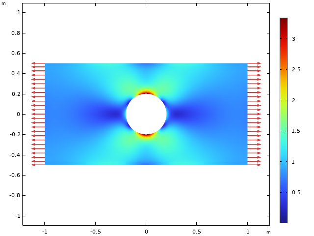
Von Mises equivalent stress, using a plane stress assumption.
Under plane stress assumptions, the transverse stress, \sigma_{z} , is zero.
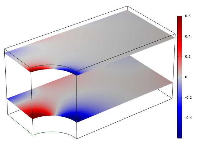
Next, we turn to a full 3D solution and look at the same object again, but with the thicknesses 0.1, 1, and 10 m, respectively. In the figure below, the transverse stress, \sigma_{z}, is plotted.
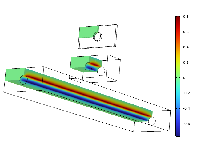
Transverse stress for three different thicknesses.
The transverse stress is negligible for the thin configuration, so the plane stress is a good assumption. For the intermediate thickness, the stress state is fully three-dimensional. With a long object, a constant transverse stress prevails, except at the ends. Note that the maximum transverse stress is 0.8 MPa, so it is by no means negligible when compared to the applied load.
Below, the transverse stress at the most stressed location at the top of the hole is studied in more detail.
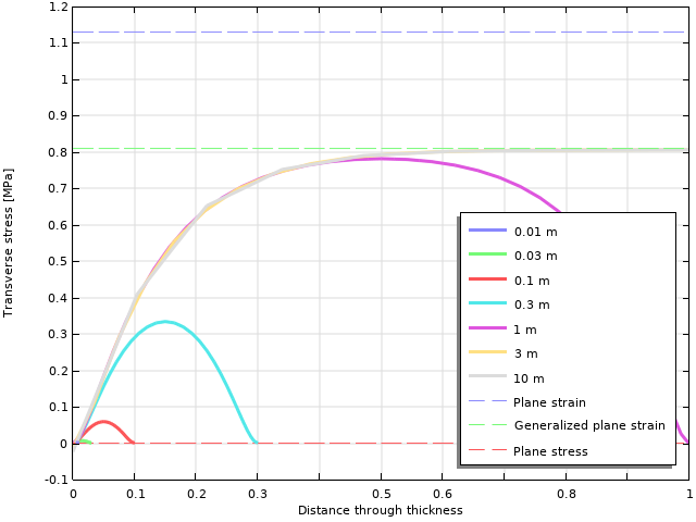
Transverse stress variation through the thickness. The parameter for the graphs is the thickness of the object.
As can be seen, as long as the thickness is 1 m or more, a peak level of about 0.8 MPa is reached. When the thickness is smaller, the maximum transverse stress drops fast.
This graph will actually help us clear out two common misconceptions:
- Just because an object is free in the transverse direction does not mean it is in a state of plane stress.
- A long object is not necessarily in a state of plane strain. This holds only if the ends are fixed.
The truth is:
- A thin object with free boundaries can be approximated by plane stress.
- A long object with free boundaries can, away from the ends, be approximated by generalized plane strain.
- An object that has a thickness comparable with the in-plane dimensions must be considered as fully 3D.
Actually, the statement that objects that are thick should be considered to be in a state of plane strain can be found almost everywhere in textbooks and online. While it is true that plane strain is a better approximation than plane stress in this situation, it is still not correct. A generalized plane strain assumption is better.
My personal guess is that since working with 2D solutions dates back to the times when many problems were solved by pen and paper, for example, using the Airy stress function, the choice stood in practice between plane stress and plane strain. With finite element software, full 3D or generalized plane strain are better options for thicker objects.
Why Do Transverse Stresses Occur?
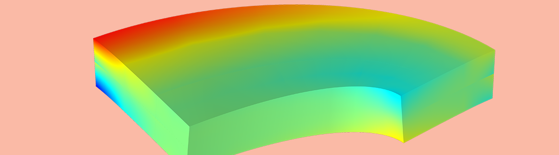
In the example above, we have seen that significant stresses develop in the transverse direction, even though the object is free to move in that direction. Why? Due to the Poisson’s ratio effect, there will be a thickness change in the out-of-plane direction. As long as there is a stress (and strain) gradient in the in-plane state, this thickness change is not uniform. At a stress concentration, like the hole in the plate, the material at the most stressed point wants to get thinner than the material in its surroundings. The neighboring material will oppose to that and try to suppress the deformation.
Variation in transverse displacement far from the free surface (bottom) and near the free surface (top). In each plane, the average displacement is set to zero.
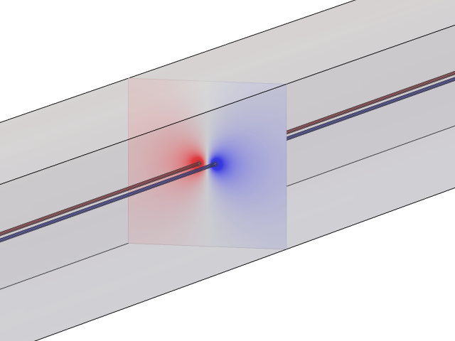
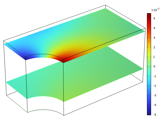
In the previous section, it was noted that the size of the transverse stress differs with distance from the free boundary. The details of the stress distribution also differ with the distance from the free surface, as illustrated in the figure below.
Distribution of transverse stress far from the free surface (bottom) and near the free surface (top). The stress fields are scaled to have the same peak value in both cut planes; the actual stress is lower close to the boundary.
Far from the free surface, the transverse stress is directly proportional to the in-plane strains \varepsilon_x+\varepsilon_y. The whole section maintains a more or less uniform thickness because of the constraint effect from the surrounding material. Close to the free surface, however, the transverse stress is instead high where there are large gradients in the in-plane strains; in this case, close to the edge of the hole.
What About In-Plane Stresses?
As long as the structure is only loaded by tractions (and not prescribed displacements), then the in-plane stress state is independent of the 2D assumption, at least for linear elasticity. That is, however, not the full story. In the figure below, the x direction stress is shown at the most stressed location at the top of the hole.
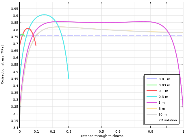
Horizontal stress variation through the thickness. The parameter for the graphs is the thickness of the object.
As can be seen, there is a significant variation through the thickness. For thin objects, the 2D value matches well, whereas for thicker objects, there is a significant difference, particularly at the free surface. This also has implications on the equivalent stresses.
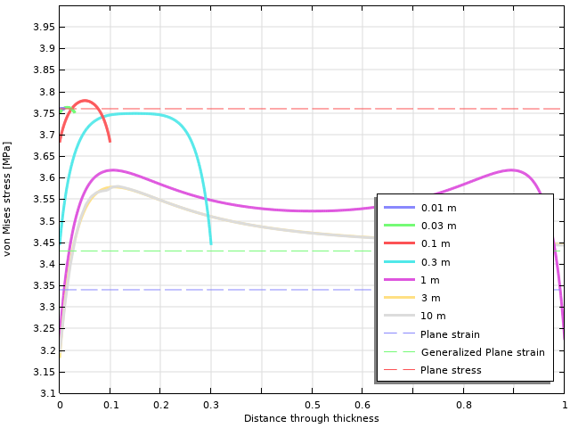
Von Mises equivalent stress variation through the thickness. The parameter for the graphs is the thickness of the object.
For thicker objects, there is a significant difference between the actual equivalent stress and any of the 2D solutions. Only in the interior of fairly thick objects, the von Mises stress will converge toward the generalized plane strain solution.
Inelastic Strains
In many cases, the difference between the three formulations is not as pronounced as in the previous example, where there is a significant stress concentration. However, there are some cases where you must be particularly observant: when inelastic strains are important. Then, it is not only the Poisson’s ratio effect on the in-plane strains that acts in the transverse direction.
Consider, for example, thermal expansion. It is usually uniform in all directions. This means that in a plane strain setting, where out-of-plane expansion is inhibited, there will be a strong buildup of transverse stress. An object that is free to expand in the xy-plane will experience a transverse stress that is \sigma_z = -E \alpha \Delta T. If you select to use a plane stress or generalized plane strain formulation, the expansion in the transverse direction is free, and this stress will not appear.
As an illustration of the importance of the 2D formulation in the case of thermal expansion, the following case is studied: A square plate with free expansion in the xy-plane is subjected to a temperature field where the temperature is proportional to x*y. The maximum temperature increase (in the upper-right corner) is 100 K. Material data for steel is used. The stress in the transverse direction is shown in the figure below.
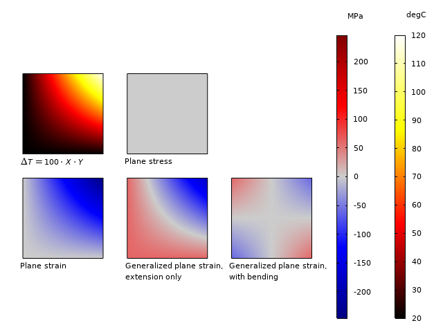
Temperature distribution and out-of-plane stress \sigma_z for different 2D assumptions.
The results show that:
- For the plane stress case, the out-of-plane expansion is free, so that no stress is induced.
- For plane strain, the whole section experiences a compressive stress, with the value \sigma_z = -E \alpha \Delta T(x,y). The stress ranges from -245 to 0 MPa.
- For generalized plane strain with pure extension, a constant stress is added, so that the average \sigma_z becomes zero. The stress ranges from -184 to 61 MPa.
- For generalized strain with bending, a linearly varying stress field is also added. The stress now ranges from -61 to 61 MPa.
A Note on Equivalent Stresses
The two most commonly used scalar stress measures are the von Mises equivalent stress and the Tresca equivalent stress. If we express them in terms of the principal stresses (\sigma_1 > \sigma_2 > \sigma_3), then
and
As can be seen, the intermediate principal stress affects the von Mises equivalent stress, but not the Tresca equivalent stress. For 2D cases, the out-of-plane stress component \sigma_z is always one of the principal stresses. For the plane stress case, it is zero. For the plane strain case, it is \sigma_z = \nu \left ( \sigma_x + \sigma_y \right ) = \nu \left ( \sigma_{1 \mathrm p} + \sigma_{2 \mathrm p} \right ) for a linear elastic material. The last expression contains the two in-plane principal stresses. If \sigma_{1 \mathrm p} and \sigma_{2 \mathrm p} have different signs, then \sigma_z is always the intermediate principal stress, and the Tresca equivalent stress is not affected by a change between plane stress and plane strain.
This invariant behavior cannot be seen for the von Mises equivalent stress because of its dependency of the intermediate principal stress.
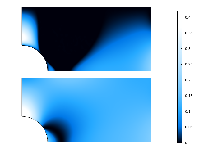
Difference between equivalent stress values under plane stress and plane strain conditions. Tresca (above) and von Mises (below). Note the large black region with zero difference in the Tresca case.
A Note on Fracture Mechanics
In fracture mechanics, it is common to analyze thick plates under the assumption of plane strain. Why is that okay, now that we have seen that generalized plane strain or full 3D are the correct options?
In this context, it is mainly the state at the crack tip that is important. The strain state at the crack tip is singular, so there is a strong tendency for the material to contract in the thickness direction. This is resisted by the surrounding material, forming a strong constraint against thickness direction displacement. Thus, the stress state close to the crack tip resembles plane strain. Actually, a plane strain solution and a generalized plane strain solution will give rather similar results close to the crack tip. This is not to say that plane strain is a good approximation everywhere in a plane cracked body. Actually, the plane strain solution will underestimate the global deformations somewhat. In most of the plate, where the stress gradients are small, plane stress is a better approximation.
1D Theories
Slender structures are often modeled using beam or truss approximations. For these cases, uniaxial theories are used. The stresses and strains in the transverse directions are not directly part of the problem formulation. If you study the details, you will, however, find an underlying assumption that there are no stresses in the transverse directions. Essentially, there are two (arbitrary) orthogonal directions in which plane stress conditions prevail. It is possible to compute the transverse strain a posteriori, should the need arise. For a linear elastic material, the definition of Poisson’s ratio can be directly used; the transverse strain is \varepsilon_T = -\nu \varepsilon_A, where \varepsilon_A is the axial strain.
As of version 6.1 of COMSOL Multiphysics, the Solid Mechanics interface is available also for 1D and 1D axisymmetric geometries. Here, you also have to make a decision about the out-of-plane behavior. In the 1D case, you can independently choose between plane stress, plane strain, and generalized plane strain in the two transverse directions. In the case of 1D axisymmetry, you have the same three options for the behavior in the thickness direction.


Part of the Settings windows for the Solid Mechanics interface in 1D and 1D axisymmetry.
Next Step
The Structural Mechanics Module, an add-on to COMSOL Multiphysics, includes specialized features and functionality for modeling plane stress and plane strain. Learn more about the module by clicking the button below:


Comments (6)
Ivar KJELBERG
May 20, 2021Hi Henrik,
Thanks again for an excellent BLOG. Indeed Structural, just as magnetic field theory and a few other Physics, are a true 3D problem, and any 2D approach is only an approximation, but as you show, with some investigations, one may still use efficiently 2D structural analysis.
And a special thanks for the “Note on Equivalent Stresses” chapter, as really the thermal stress buildup in 2D that one may notice has surprised, and given quite some white hear, to more than one of us, but once understood, it’s rather “evident”.
Sincerely
Ivar
Jay Puckett
May 27, 2021Very nice article. Good presentation about a lot of topics related to plane-stress and -strain. A lot is presented in a succinct article.
Belouadah AbdelHakim
June 3, 2021very useful article thank you a lot
CHeolWoong Kim
July 23, 2021Thanks for a great article.
I have a question about the plane stress in COMSOL.
Could I find how the extra variable(e_zz) is implemented at the COMSOL desktop?
When I saw “Equation view” under “Linear Elastic Material”, the shape function for wZ was only found.
But, in the COMSOL desktop, I cannot find any equation which e_zz should satisfy.
Sincerely
Kim
Henrik Sönnerlind
July 23, 2021 COMSOL EmployeeThe degree of freedom wZ represents the (partial) derivative dw/dZ. For a geometrically linear study, this is the same as the transverse strain e_zz.
This strain is then used in a full 3D constitutive relation; that is it contributes to the 3D stress tensor S. Finally, the full 3D weak expression is used for equilibrium, S:test(e)=0. One of the terms in this sum is S_zz*test(e_zz). Since there are no loads acting in the Z direction, this equation enforces S_zz = 0.
Note that is only ascertains that the transverse stress in zero in the weak (finite element) sense. This is why you sometimes can see small (but negligible) stresses in the transverse direction.
CHeolWoong Kim
July 24, 2021Thank you so much!
I fully understand what you said.